2 Introduction

You can label chapter and section titles using {#label} after them, e.g., we can reference Chapter 2. If you do not manually label them, there will be automatic labels anyway, e.g., Chapter 4.

2.1 Figures and Tables

2.1.1 Figures

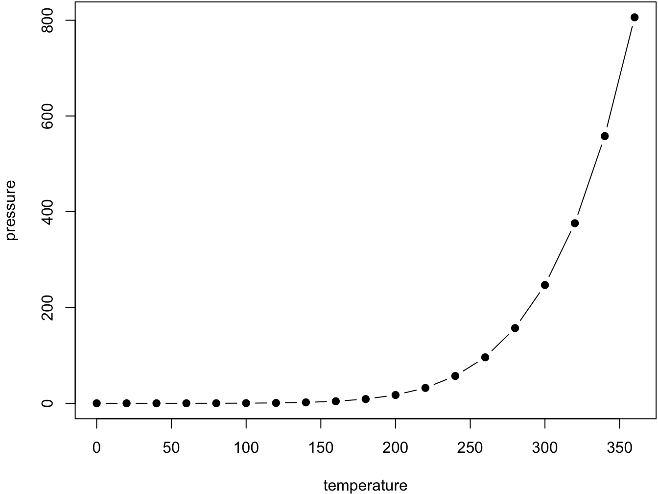
Figures and tables with captions will be placed in figure and table environments, respectively.

par(mar = c(4, 4, .1, .1))
plot(pressure, type = 'b', pch = 19)

Figure 2.1: Here is a nice figure!

2.1.2 Tables

Reference a figure by its code chunk label with the fig: prefix, e.g., see Figure 2.1. Similarly, you can reference tables generated from knitr::kable(), e.g., see Table 2.1.

knitr::kable(
  head(iris, 20), caption = 'Here is a nice table!',
  booktabs = TRUE
)

Table 2.1: Here is a nice table!
Sepal.Length	Sepal.Width	Petal.Length	Petal.Width	Species
5.1	3.5	1.4	0.2	setosa
4.9	3.0	1.4	0.2	setosa
4.7	3.2	1.3	0.2	setosa
4.6	3.1	1.5	0.2	setosa
5.0	3.6	1.4	0.2	setosa
5.4	3.9	1.7	0.4	setosa
4.6	3.4	1.4	0.3	setosa
5.0	3.4	1.5	0.2	setosa
4.4	2.9	1.4	0.2	setosa
4.9	3.1	1.5	0.1	setosa
5.4	3.7	1.5	0.2	setosa
4.8	3.4	1.6	0.2	setosa
4.8	3.0	1.4	0.1	setosa
4.3	3.0	1.1	0.1	setosa
5.8	4.0	1.2	0.2	setosa
5.7	4.4	1.5	0.4	setosa
5.4	3.9	1.3	0.4	setosa
5.1	3.5	1.4	0.3	setosa
5.7	3.8	1.7	0.3	setosa
5.1	3.8	1.5	0.3	setosa

You can write citations, too. For example, we are using the bookdown package (Xie 2021) in this sample book, which was built on top of R Markdown and knitr (Xie 2015).

2.2 Something else

Placeholder text.

1 Prerequisites

3 Literature